Are you searching for an easy to interpret, yet powerful Machine Learning algorithm? It does not matter if you are a newcomer or an experienced one, the Decision tree is the way to go.
Or maybe if you are looking for an algorithm that can help you to improve your model accuracy or compete in a hackathon then a decision tree is a must. As decision trees are building blocks of the most popular algorithms like Random Forest, XGBoost, LightGBM, and Catboost.
If you are interested in hackathons but do not know where to find them. You can follow this brilliant article “Top 25 Machine Learning & AI Hackathons for Anyone to Move to Data Science!“ written by Vetrivel PS.
So, you can imagine why learning about decision trees is really important.

Are you confused and asking where I start and how I processed? If so, you have reached the perfect place.
This article will help you to understand and apply the Decision Tree and allow you to make great progress in your career.
What is a Decision Tree?
A Decision Tree algorithm is a supervised learning algorithm used for making decisions by splitting a problem into smaller, more manageable parts. It’s a flowchart-like structure in which the tree is created at the root node and then splitting the data into groups called internal nodes. Each internal nodes use to test attributes and each leaf node represents a class label.
A decision tree algorithm is a powerful tool that can be used for both classification and regression. This can also be used to make predictions from complex datasets in a top-down, greedy approach that splits the dataset into subsets based on an attribute value test.
For example, you recently moved to a new city and are confused about buying a house or renting one. Let’s create a decision tree that can help you to make a decision. A decision always starts with a root node and ends with leaves nodes. So, for this example, our root node could be “Are you planning to stay for more than 5 years”.

If you do not want to go through the theory and directly want to see the implementation of the decision tree using the scikit-learn in python click here.
Jargon Alert
Root Nodes – The very top node which represents the beginning of a tree is called the Root Node.
Decision Nodes/Internal Nodes/Branches – When a node splits into two or more sub-nodes is called a decision node. Internal Nodes have arrows pointing to them and arrows pointing away from them.
Leaf node/ Leaves Nodes / Terminal Node – The Nodes where splitting is not possible are called leaves nodes
Sub-tree – A small portion of a tree is called a sub-tree. Used to explain a complex tree by dividing it into multiple sub-trees.
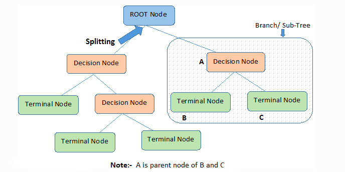
When applying a decision tree this is the Basic Algorithm
- Pick the best feature which splits the data based on the attributes.
- Split the data into subsets based on the selected feature.
- Repeat steps 1 and 2 on each subset until you find leaf nodes in all branches of the tree.
Assumption while creating Decision Tree
Below are some of the assumptions we make while using Decision Tree:
- In the beginning, the whole training set is considered as the root.
- Features values are preferred to be categorical. If the values are continuous then they are discretized prior to building the model.
- Records are distributed recursively on the basis of attribute values.
- Order to place attributes as root or internal node of the tree is done by using some statistical approach.
Decision Tree Cheatsheet
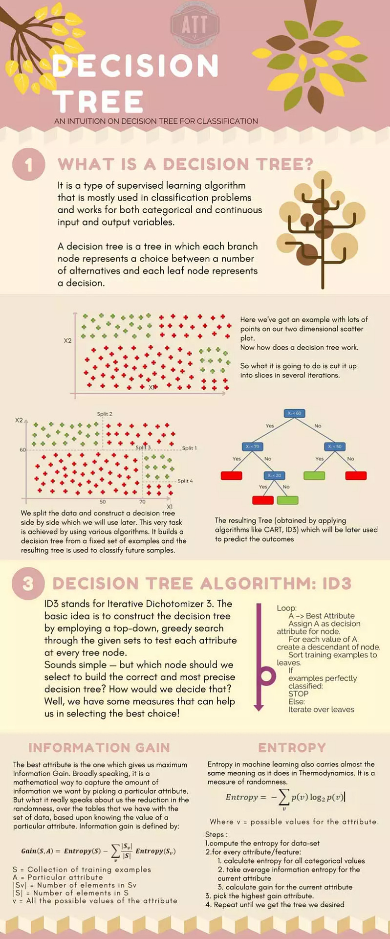
Implementing the decision tree algorithm
Decision trees follow the Sum of Product(SOP) representation which is also known as the Disjunction Normal Form. If we normalize a logical formula in boolean mathematics is called Disjunctive Normal Form(DNF). The propositional operators of DNF are: AND, OR, and NOT.
For a class, every branch from the root of the tree to the leaves node having the same class is the conjunction(product) of values, different branches ending in that class form a disjunction(sum).
While implementing the decision tree algorithm, the primary challenge is to identify the root and decision nodes attribute of the tree. If we randomly select any node as the root node it may give us really low accuracy. To get the best result we use a technique called Attributes Selection Measure(ASM). Researchers suggested different criteria like the Gini index to find the best attribute for the root node at each level.
These criterion values are calculated for each attribute and then sorted. Attribute with high value is placed at the root.
Note: While we are working with categorical attributes we consider information gain as a criterion and for continuous attributes we consider the Gini index.
The popular attribute selection measures:
- Categorical Target Variable
- Entropy
- Information gain
- Gini index
- Chi-Square
- Continuous Target Variable
- Reduction in Variance
Decision Tree Splitting Methods
Entropy
Entropy is a measure of the disorder or randomness in the information being processed. A node with entropy value 0 is called a “Pure Node”. While constructing a decision tree our goal is to split the tree until we reach all the pure nodes. Entropy ranges from 0 to 1. The higher the entropy, the harder it becomes to find a conclusion from the information.
Flipping a coin is an example of an action where the information is random and has an equal 50% chance of heads or tails.
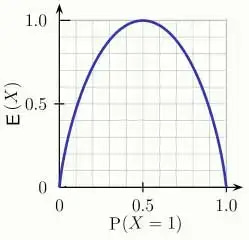
In the graph, we can see the entropy E(X) is zero when the probability is either 0 or 1. The entropy is maximum when the probability is 0.5. Because that time the randomness will be maximum and it will become harder to find a conclusion.
The formula for calculating entropy:

In a much simpler way, we can conclude that:

Where S=Total number of samples
P(yes)=Probability of Yes
P(No)=Probability of No
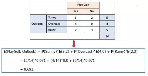
Mathematically Entropy for multiple attributes is represented as:

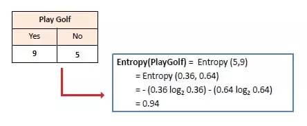
Consider you want to predict whether your friend is going to join you to play a game of golf or not. This could depend on a few factors like outlook. temp, humidity, and wind. From the historical data, we could get a table like this.
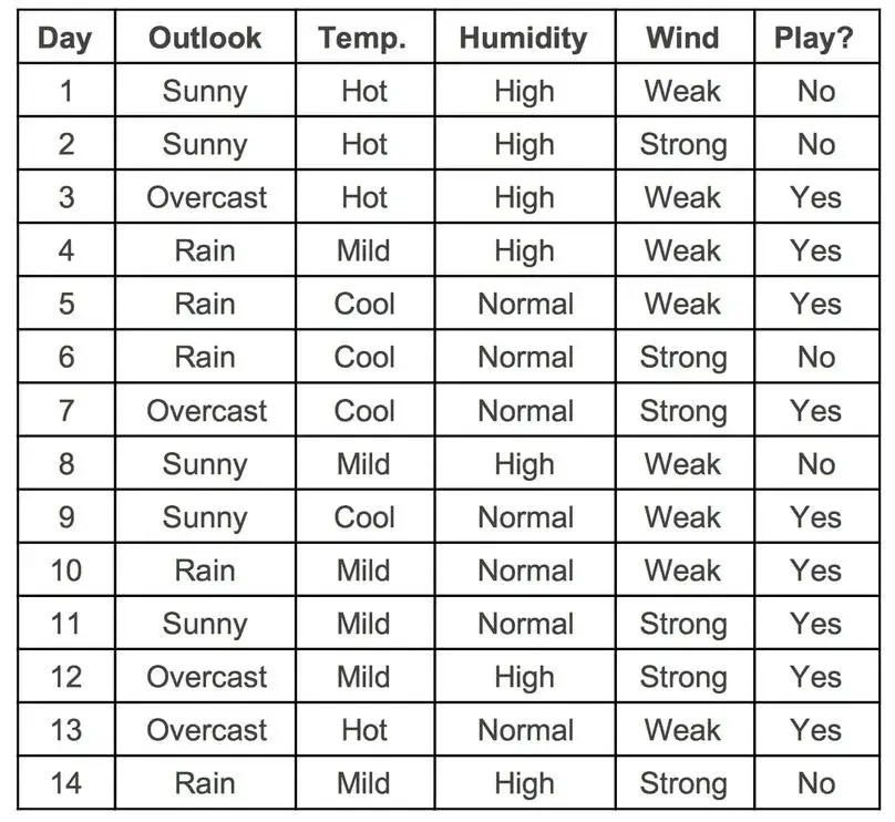
Mathematically Entropy for 1 attribute is represented as:
Mathematically Entropy for multiple attributes is represented as:
Information Gain
By using information gain as the criterion, we try to get an estimate of the information contained in each attribute. It favors smaller partitions with distinct values. We decide on partitioning based on the partition giving the highest information gain and the smallest entropy.
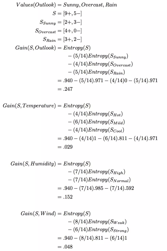
There are two steps for calculating information gain for a tree:
- Calculate the entropy of the target attribute
- Calculate entropy for every attribute and subtract this from the entropy of the target. the result is information gain.
Formula for calculating information gain:
Information Gain = Entropy(S) – [(Weighted Avg) * Entropy(each feature)]
In a much simpler way, we can conclude that:

Gini Index
The Gini index was stated originally by Leo Breiman in 1984. It is based on Gini impurity. This helps us to understand the amount of uncertainty a node has. Using Gini we can calculate the probability of correctly labeling; if an attribute was randomly labeled according to the distribution of labels. Gini index ranges from 0 to 1, where the lower the Gini impurity, the higher the homogeneity of the node (also indicates less uncertainty). Like Entropy, a node with 0 Gini impurity is called a “Pure Node”.

Chi-Square
It’s one of the oldest methods of tree classification. it measures the statical significance of differences between the child and parent nodes. We measure it using the sum of squares of the standardized discrepancies between the observed and expected frequencies of the target variable for each node.
Using the chi-square method we can do numerous splits at a single node, resulting in higher accuracy. Also, we should keep in mind that the higher the Chi-square value, the greater the statistical significance of the difference between child and parent node
Chi-Square value is:

You can watch it below video explaining chi-square with an example:
Reduction in Variance
When the target variable is a continuous value (regression problem). Reduction in Variance is a method used for splitting the nodes in a decision tree. It is called reduction in variance as the feature with lower variance is selected as the criteria to split into child nodes. The algorithm uses the standard formula of variance to choose the best split. If a node is entirely homogeneous then the variance is zero. Our target will be to archive homogeneous leaves nodes.

Why Gini Impurity is better than Entropy?
To give this answer we analyzed training time and F-Scores. We tested on different datasets where all of these datasets have 10 features. Based on the features, they can be grouped into 4 different groups informative, redundant, repeated, or random.
| Dataset 1 | Dataset 2 | Dataset 3 | Dataset 4 | |
|---|---|---|---|---|
| Informative | 100% | 30% | 30% | 30% |
| Redundant | 0 | 70% | 0 | 0 |
| Repeated | 0 | 0 | 70% | 0 |
| Random | 0 | 0 | 0 | 70% |
In the below graphs, the x-axis is the number of the datasets, and the y-axis is the training time.
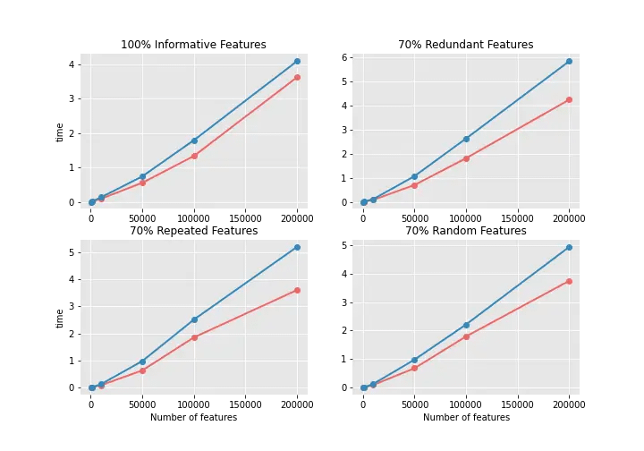
As you can see training time using entropy is much higher. For Redundant features, the training time is even 50% longer than using the Gini impurity test. If we increase the size of the dataset the difference between training will be more noticeable.
Computationally, entropy is more complex since it makes use of logarithms and consequently, the calculation of the Gini Index will be faster. On other hand, the entropy criterion will manage to give slightly better results.
However, as the results are so similar, it does not seem to be worth the time invested in training when using the entropy criterion.
How to deal with overfitting in a decision tree
Overfitting is a general problem we have to deal with in almost every machine learning algorithm out there. Overfitting means when the model ends up memorizing the training data instead of generalizing it. The decision tree does not have any exceptions, it also faces overfitting when the tree has too many branches. The main reason for too many branches could be outliers and irregularities in data. This can lead to good performance in training data but poor performance on unseen data.
There are a few ways to resolve overfitting in a decision tree.
- Pruning
- Stopping criterion
Pruning:
Pruning simply means trimming off extra branches in a tree that is not necessary. By the approach, we can divide pruning into two types
- Pre-pruning
- Post-pruning
Pre-pruning
In pre-pruning, by using a threshold value we stop the construction a bit early. Basically, it’s not going to split a node if its goodness measure is below a threshold value. We can also pre-pruning using Hyperparameter tunning.
Post-pruning
From the name you can guess this technique is applied after the construction of the decision tree. This is also known as backward pruning. We use cross-validation data to check the effect after pruning and we will control the branches of the tree using cost_complexity_prunning.
Stopping criterion
Bigger the decision trees, the more the complexity. One method to reduce this complexity is by not allowing the trees to reach the end and stopping them in between through some stopping criteria. If we continue to grow the tree fully until each leaf node reaches the lowest impurity then the tree could have been overfitted.
On the opposite of this if we stop splitting too early error into training data is not sufficiently high and performance will suffer. We can stop the tree splitting through some stopping criteria. These criteria are
- Information gain is very small
- Impurity gets increased
- Setting the maximum depth of the tree
Algorithms to build decision trees
Algorithm selection is always based on the type of target variable. At the core, they give you a procedure to decide which questions to ask and when.
Some of the popular algorithms used in decision trees are:
- ID3 (Extensive of D3)
- C4.5 ( Successor of ID3)
- CART (Classification and Regression Tree)
- CHAID (Chi-square automatic interaction detection performs multi-level splits when computing classification trees)
- MARS (Multivariate adaptive regression splines)
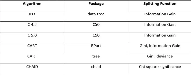
Scikit-learn uses an optimized version of the CART algorithm and this algorithm uses the Gini index.
Advantages and Disadvantages of Decision Tree Algorithm
Advantages of Decision Tree Algorithm
- Decision Trees are fast. They can quickly process large amounts of data, making them ideal for decision-making applications.
- Decision Trees are easy to explain. They are simply a series of if-else conditions.
- Decision Trees are versatile. They can handle both numerical and categorical data.
Disadvantages of Decision Tree Algorithm
- Trees can be unstable. Even a small change in the dataset can result in a very different unstable tree structure which can cause variance.
- There is a high probability of overfitting the decision tree.
- When there are many class labels, they can be computationally expensive to train. If we compare decision trees with linear models decision trees can require a lot of memory and time to train for large complex data.
- Decision trees create underfit trees if some classes are unbalanced. Also if there are greater no. of categories it gives a biased response for those attributes.
- They are often suffering from inaccuracy. Other machine learning methods introduced like Random forest, XGBoost, and neural networks can ofter perform better.
Decision Tree Python Implementation using Scikit-learn
For this example, we using UCI, Heart Disease Dataset. You can download the dataset by clicking here.
#imports
import numpy as np
import pandas as pd
import matplotlib.pyplot as plt
import seaborn as sns
Read Data
df = pd.read_csv('processed.cleveland.data',header=None)
df.columns = [
    'age',
    'sex',
    'cp',
    'restbps',
    'chol',
    'fbs',
    'restecg',
    'thalach',
    'exang',
    'oldpeak',
    'slope',
    'ca',
    'thal',
    'hd',
]

df.head()

Data contains;
- age – age in years
- sex – (1 = male; 0 = female)
- cp – chest pain type
- restbps – resting blood pressure (in mm Hg on admission to the hospital)
- chol – serum cholesterol in mg/dl
- fbs – (fasting blood sugar > 120 mg/dl) (1 = true; 0 = false)
- restecg – resting electrocardiographic results
- thalach – maximum heart rate achieved
- exang – exercise-induced angina (1 = yes; 0 = no)
- oldpeak – ST depression induced by exercise relative to rest
- slope – the slope of the peak exercise ST segment
- ca – number of major vessels (0-3) colored by fluoroscopy
- thal – 3 = normal; 6 = fixed defect; 7 = reversible defect
- hd – have disease or not (1=yes, 0=no)
print(f"Dataset Shape :- \n {df.shape})"

## Output
"""
Dataset Shape:-
 (303, 14)
"""
Exploratory Data Analysis (EDA)
# Heart Disease Frequency for Ages

pd.crosstab(df.age,df.hd).plot(kind="bar",figsize=(20,6))
plt.title('Heart Disease Frequency for Ages')
plt.xlabel('Age')
plt.ylabel('Frequency')
plt.show()

# Heart Disease Frequency for Sex

pd.crosstab(X.sex,y.hd).plot(kind="bar",figsize=(15,6),color=['#0da62e','#e60303' ])
plt.title('Heart Disease Frequency for Sex')
plt.xlabel('Sex (0 = Female, 1 = Male)')
plt.xticks(rotation=0)
plt.legend(["Haven't Disease", "Have Disease"])
plt.ylabel('Frequency')
plt.show()
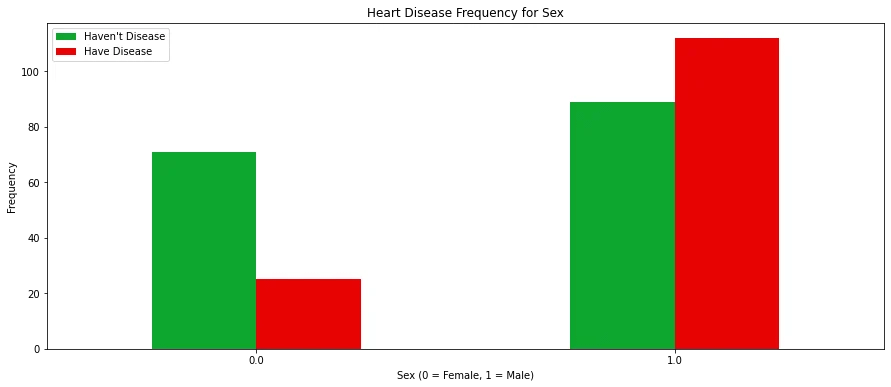
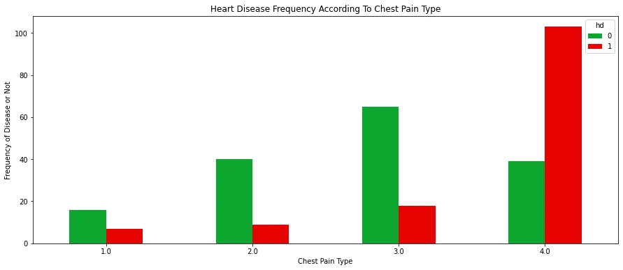
# Heart Disease Frequency According To Chest Pain Type

pd.crosstab(X.cp,y.hd).plot(kind="bar",figsize=(15,6),color=['#0da62e','#e60303' ])
plt.title('Heart Disease Frequency According To Chest Pain Type')
plt.xlabel('Chest Pain Type')
plt.xticks(rotation = 0)
plt.ylabel('Frequency of Disease or Not')
plt.show()
# Heart Disease Frequency According To FBS

pd.crosstab(X.fbs,y.hd).plot(kind="bar",figsize=(15,6),color=['#0da62e','#e60303' ])
plt.title('Heart Disease Frequency According To FBS')
plt.xlabel('FBS - (Fasting Blood Sugar > 120 mg/dl) (1 = true; 0 = false)')
plt.xticks(rotation = 0)
plt.legend(["Haven't Disease", "Have Disease"])
plt.ylabel('Frequency of Disease or Not')
plt.show()

Checking null or nan values
We can check the data types and at the same time, the number of non-null values of all features by using the info() method of pandas. If you only want to check the data type of the features then you can use dtypes.
See the result of dataset info();
print(f"Dataset info :- \n {df.info()}")

## Output
"""
<class 'pandas.core.frame.DataFrame'>
RangeIndex: 303 entries, 0 to 302
Data columns (total 14 columns):
 #   Column   Non-Null Count  Dtype
---  ------   --------------  -----
 0   age      303 non-null    float64
 1   sex      303 non-null    float64
 2   cp       303 non-null    float64
 3   restbps   303 non-null    float64
 4   chol     303 non-null    float64
 5   fbs      303 non-null    float64
 6   restecg  303 non-null    float64
 7   thalach  303 non-null    float64
 8   exang    303 non-null    float64
 9   oldpeak  303 non-null    float64
 10  slope    303 non-null    float64
 11  ca       303 non-null    object
 12  thal     303 non-null    object
 13  hd       303 non-null    int64
dtypes: float64(11), int64(1), object(2)
memory usage: 33.3+ KB
"""
it provides all information about our dataset, such as
- Total number of samples or rows
- Column names
- Number of non-null values
- The data type of each column
Our dataset doesn’t have any null values because the total number of features is 303 ranging from 0 – 302; all features have the same number of samples/rows.
We “ca” should contain the number of major vessels(0-3) which should be float or int. But it’s datatype showing object. Let’s explore it.
print(f"Unique values of ca variable :- \n {df['ca'].unique()}")

## Output
"""
Unique values of ca variable :-
array(['0.0', '3.0', '2.0', '1.0', '?'], dtype=object)
"""
As we can see ca have missing values pointed by ‘?’. Next, we are going to do the same for thal variables and also we are going to check how many missing values are there.
# print out the number of rows that contain missing values

len(df.loc[(df['ca']=='?')
|
(df['thal']=='?')])

## Output
"""
6
"""
Creating a mask and dropping missing values.
df = df.loc[(df['ca'] != '?')
&
(df['thal'] != '?')]
As you can see all of the 6 missing values are dropped.
print(f"Dataset Shape :- \n {df.shape})"

## Output
"""
Dataset Shape:-
 (297, 14))
"""
Splitting the dataset into dependent and independent variables
Now we will take all independent columns (the target column is dependent and the remaining all are independent columns to each other), as X and the target variable as y.
# Features and target creations
X = df.drop(['hd'],axis=1).copy()
y = df[['hd']].copy()
Format the Data: One Hot Encoding
The preferred data type of each should be like this.
- age – Float
- sex – Category
- 0 = female
- 1 = male
- cp, chest pain – Category
- 1 = typical angina
- 2 = atypical angina
- 3 = non-anginal pain
- 4 = asymptomatic
- restbp, resting blood pressure(in mm Hg) – Float
- chol, serum cholesterol in mg/dl – Float
- fbs, fasting blood sugar – Category
- 0 =>= 120 mg/dl
- 1 =< 120 mg/dl
- restecg, resting electrocardiographic results – Category
- 0 = normal
- 1 = having ST-T wave abnormality
- 2 = showing probable or definite left venticular hypertrophy
- thalach, maximum heart rate achieved – Float
- exang, exercise induced angina – Category
- 0 = no
- 1 = yes
- oldpeak, St depression induced by exercise relative to rest – Float
- Slope, the slope of the peak exercise ST segment – Category
- 1 = unsloping
- 2 = flat
- 3 = downsloping
- ca, number of major vessels(0-3) colored by fluoroscopy – Float
- Thal, thalium heart scan – Category
- 3 = normal
- 6 = fix defect
- 7 = reversible defect
But as you can see current data types of our data.
print(f"Dataset info :- \n {df.info()}")

## Output
"""
<class 'pandas.core.frame.DataFrame'>
RangeIndex: 303 entries, 0 to 302
Data columns (total 14 columns):
 #   Column   Non-Null Count  Dtype
---  ------   --------------  -----
 0   age      303 non-null    float64
 1   sex      303 non-null    float64
 2   cp       303 non-null    float64
 3   restbps   303 non-null    float64
 4   chol     303 non-null    float64
 5   fbs      303 non-null    float64
 6   restecg  303 non-null    float64
 7   thalach  303 non-null    float64
 8   exang    303 non-null    float64
 9   oldpeak  303 non-null    float64
 10  slope    303 non-null    float64
 11  ca       303 non-null    object
 12  thal     303 non-null    object
 13  hd       303 non-null    int64
dtypes: float64(11), int64(1), object(2)
memory usage: 33.3+ KB
"""
Two popular methods to do one-hot encoding is ColumnTransformer() from sci-kit learn and get_dummies() from pandas. Here we are going to use get_dummies().
X_encoded = pd.get_dummies(X, columns=['cp',
'restecg',
'slope',
'thal'])

X_encoded.head()
Let’s see what are the unique values we are having for the target variable. We know “hd” is the target variable, and the remaining all are features of our dataset.
print(f"Unique values of target variable :- \n {df['hd'].unique()}")

## Output
"""
Unique values of target variable :-
 [0 2 1 3 4]
"""
Here we only want to detect if someone has a change of heart disease or not. For this example, we are not worried about the degree of heart disease. So, we are going to convert 2,1,3,4 as 1.
y_not_zero_index = y > 0 #getting the index of non zero values
y[y_not_zero_index] = 1
Now, we need to split the whole dataset into train and test datasets. Training data is used at the time of building the model and a test dataset is used to evaluate trained models.
By using the train_test_split method from the sklearn library we can do this process of splitting the dataset into 70% train and 30% test sets.
#split the data into train and testing sets
from sklearn.model_selection import train_test_split

X_train, X_test, y_train, y_test = train_test_split(X_encoded, y, random_state=29,test_size=0.3)
print(X_train.shape)
print(X_test.shape)
print(y_train.shape)
print(y_test.shape)

## Output
"""
(207, 22)
(90, 22)
(207, 1)
(90, 1)
"""
Building Heart Disease Detection using Machine Learning algorithm
Now our dataset is ready for building models. Let’s jump to the development of a preliminary model using the machine learning algorithm decision tree.
Preliminary Decision tree algorithm Implementation using python sklearn library
## Building decision tree
from sklearn.tree import DecisionTreeClassifier
from sklearn.metrics import confusion_matrix
from sklearn.metrics import classification_report

# initialize object for DecisionTreeClassifier class
dt_classifier  = DecisionTreeClassifier(random_state=29)
# train model by using fit method
print("Model training starts........")
dt_classifier.fit(X_train,y_train)
print("Model training completed")
acc_score = dt_classifier.score(X_test, y_test)
print(f'Accuracy of model on test dataset :- {acc_score}')

# predict result using test dataset
y_pred = dt_classifier.predict(X_test)
# confusion matrix
print(f"Confusion Matrix :- \n {confusion_matrix(y_test, y_pred)}")
# classification report for f1-score
print(f"Classification Report :- \n {classification_report(y_test, y_pred)}")

# Output

"""
Model training starts.
Model training completed
Accuracy of model on test dataset :- 0.7333333333333333
Confusion Matrix :-
 [[32 10]
 [14 34]]
Classification Report :-
               precision    recall  f1-score   support

           0       0.70      0.76      0.73        42
           1       0.77      0.71      0.74        48

    accuracy                           0.73        90
   macro avg       0.73      0.74      0.73        90
weighted avg       0.74      0.73      0.73        90
"""
Now, let’s visualize the decision tree to understand the tree structure.
plt.figure(figsize=(20,10))
plot_tree(dt_classifier,
filled=True,
rounded=True,
class_names=['No HD', 'HD'],
feature_names=X_encoded.columns);
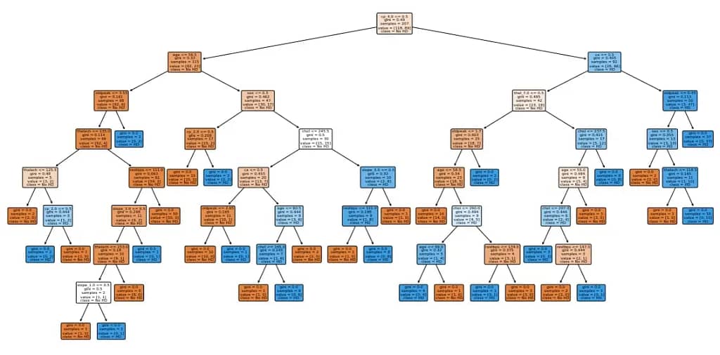
Cost complexity Pruning part 1: Visualize alpha
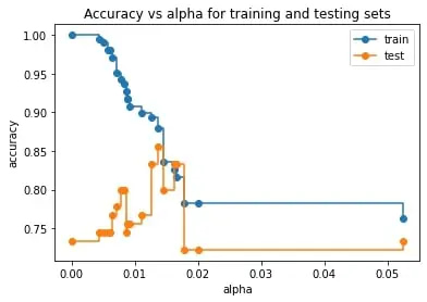
There are a lot of parameters like max_depth, and min_samples that reduce overfitting. However, pruning a tree with cost complexity pruning can simplify the whole process of finding a smaller tree that improves the accuracy of the testing dataset.
Pruning a decision tree is all about finding the right value for the pruning parameter alpha, which controls how little or how much pruning happens.
We omit the maximum value of alpha with ccp_alphas = ccp_alphas[:-1] as it prunes all leaves, leaving us with only a root instead of a tree.
train_scores = [clf_dt.score(X_train,y_train) for clf_dt in clf_dts]
test_scores = [clf_dt.score(X_test,y_test) for clf_dt in clf_dts]

fig, ax = plt.subplots()
ax.set_xlabel('alpha')
ax.set_ylabel('accuracy')
ax.set_title('Accuracy vs alpha for training and testing sets')
ax.plot(ccp_alphas,train_scores, marker='o', label='train',drawstyle='steps-post')
ax.plot(ccp_alphas,test_scores, marker='o', label='test',drawstyle='steps-post')
ax.legend()
plt.show()
Cost complexity pruning part 2: cross-validation for finding the best alpha
The graph we just drew suggested one value for alpha 0.014, but another set of data might suggest another optimal value.
We will do this by using the cross_val_score() function to generate different training and testing datasets then train and test the tree with the datasets.
clf_dt = DecisionTreeClassifier(random_state=42,ccp_alpha=0.014)

#we are creating 5-fold cross validation as we don't have lots of data
scores = cross_val_score(clf_dt, X_train, y_train, cv=5)
df = pd.DataFrame(data={'tree':range(5),'accuracy':scores})

df.plot(x='tree',y='accuracy', marker='o', linestyle='--')
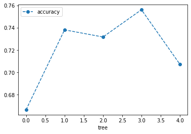
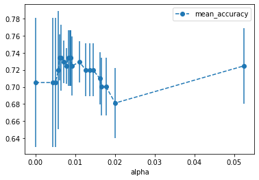
The graph above shows that using different Training and testing data with the same alpha resulted in different accuracies, suggesting that alpha is sensitive to the datasets. So instead of picking a single train dataset and signal testing dataset, let’s use cross-validation to find the optimal value for ccp_alpha.
alpha_loop_values = [] #store the results

for ccp_alpha in ccp_alphas:
    clf_dt = DecisionTreeClassifier(random_state=42, ccp_alpha=ccp_alpha)
    scores = cross_val_score(clf_dt, X_train, y_train, cv=5)
    alpha_loop_values.append([ccp_alpha,np.mean(scores),np.std(scores)])


#Now we can draw a graph of mean and standard deviations of the scores
alpha_results = pd.DataFrame(alpha_loop_values,
columns=['alpha','mean_accuracy','std'])

alpha_results.plot(x='alpha',
y= 'mean_accuracy',
yerr='std',
marker='o',
linestyle='--')
ideal_ccp_alpha = alpha_results[(alpha_results['mean_accuracy']==max(alpha_results["mean_accuracy"]))]['alpha']

ideal_ccp_alpha = float(ideal_ccp_alpha)

print(f"Ideal ccp alpha:- \n {ideal_ccp_alpha}")

# Output

"""
Ideal ccp alpha:- 0.734262
"""
Building, Evaluating, Drawing in the Final Classification Tree
clf_dt_pruned = DecisionTreeClassifier(random_state=42,
ccp_alpha=ideal_ccp_alpha)
clf_dt_pruned = clf_dt_pruned.fit(X_train, y_train)

plot_confusion_matrix(clf_dt_pruned,X_test,y_test, display_labels=['No HD', 'HD'])
print(f"Classification Report :- \n {classification_report(y_test, y_pred)}")

# Output

"""
Classification Report :-
               precision    recall  f1-score   support

           0       0.72      0.79      0.75        42
           1       0.80      0.73      0.76        48

    accuracy                           0.76        90
   macro avg       0.76      0.76      0.76        90
weighted avg       0.76      0.76      0.76        90
"""
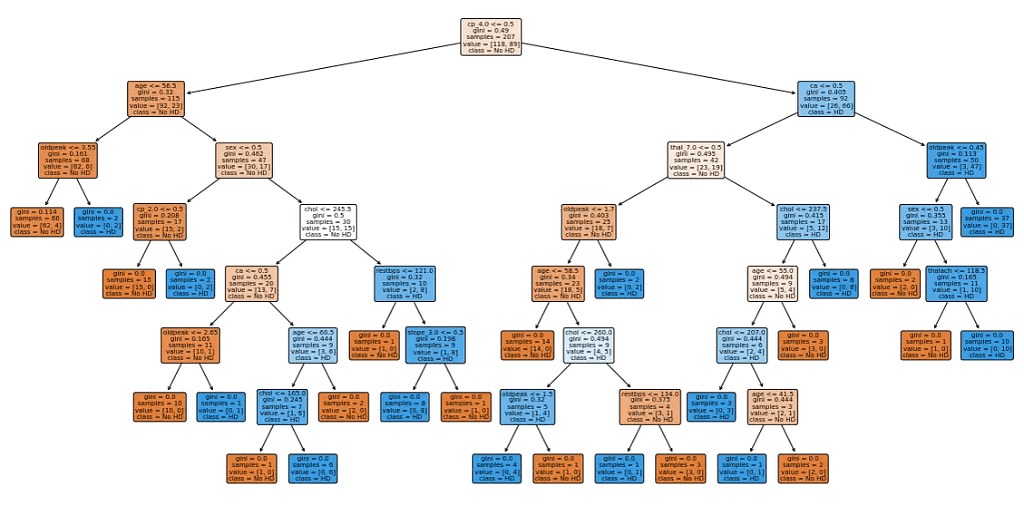
Now, let’s visualize the decision tree to understand the tree structure.
plt.figure(figsize=(20,10))
plot_tree(clf_dt_pruned,
filled=True,
rounded=True,
class_names=['No HD', 'HD'],
feature_names=X_encoded.columns);
Accuracy comparison between the two models.
acc = dt_classifier.score(X_test, y_test)*100
print("Preliminary Decision Tree Test Accuracy {:.2f}%".format(acc))

acc = clf_dt_pruned.score(X_test, y_test)*100
print("Pruned Decision Tree Test Accuracy {:.2f}%".format(acc))

# Output

"""
Preliminary Decision Tree Test Accuracy 73.33%

Pruned Decision Tree Test Accuracy 75.56%
"""
Here we have to discuss a few terms and formulae related to the confusion matrix. Using the confusion matrix we can measure the effectiveness of our model and also we can also get a better idea of what types of errors it’s making.
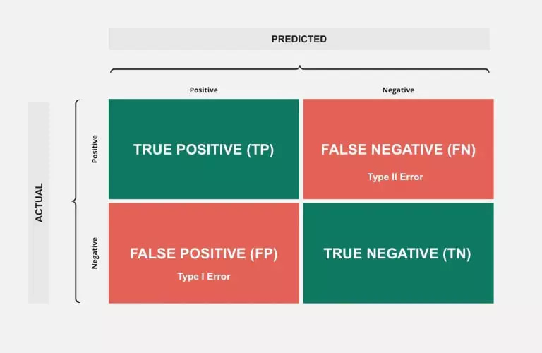
- True Positive (TP):-
The number of positive labels is correctly predicted by trained models. This means the number of Class-1 samples is correctly predicted as Class-1.
- True Negative (TN):-
The number of negative labels was correctly predicted by trained models. This means the number of Class-0 samples is correctly predicted as Class-0.
- False Positive (FP):-
The number of positive labels is incorrectly predicted by trained models. This means the number of Class-1 samples was incorrectly predicted as Class-0.
- False Negative (FN):-
The number of negative labels is incorrectly predicted by trained models. This means the number of Class-0 samples was incorrectly predicted as Class-1.
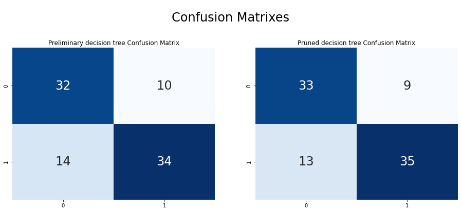
Now we are creating confusion matrixes based on preliminary and pruned decision tree models.
Conclusion
Finally, our model gives a test accuracy of 75.56% by using pruned decision trees. Which is an increment of 2% from the preliminary tree. By applying additional data preprocessing techniques or using another model like Random Forest, Support Vector Machines (SVM), and k-nearest neighbors we can get a better result.
REFERENCES:
- Decision Tree Tutorials & Notes | Machine Learning | HackerEarth
- Simonwardsjones
- Scikit-learn, Decision trees
- kdnuggets/2020/01/decision-tree
- Complete Flow of Decision Tree Algorithm
- Decision Trees and Splitting Functions (Gini, Information Gain and Variance Reduction) | by Subha Ganapathi | Nerd For Tech | Medium
- Machine Learning Recipes with Josh Gordon
If you found this article informative, then please share it with your friends and comment below with your queries or thoughts.


whoah this blog is wonderful i really like reading your articles. Keep up the great paintings! You realize, a lot of people are hunting round for this info, you could help them greatly.
I have read so many posts about the blogger lovers however this post is really a good piece of writing, keep it up